How to update a belief when the evidence changes

The report says "positive." The test detects nine out of ten cases of a certain disease. Does that mean a person with a positive result has the disease with ninety percent probability?

That information alone is not enough. We also need the frequency of the disease in the group under study, and the frequency of positive results among people who do not have that disease.

Take a hypothetical example. One person in a hundred in a defined population has the disease. We pick a person at random and have no further information about that person's health, so before seeing the result we take the probability of disease to be 1 percent. Suppose the test is also positive for 5 percent of people without the disease. Under those assumptions, a positive result raises the assessed probability to about 15.4 percent. In a moment we will see where that number comes from.

That is a large change in the assessment, even though the absence of the disease remains more probable than its presence. The result itself did not change the person's health. It changed our assessment of that health.

The distinction is useful far beyond medicine. It applies to scientific discoveries, forecasts, fraud detection, and everyday news reading. Evidence can speak for a hypothesis without yet showing that the hypothesis outweighs a competing explanation.

In the first article in this series, we looked at how single results become well-supported knowledge. The question now is how to update a belief when the evidence changes: how much should we revise our assessment when new information arrives?

Two questions that are easy to confuse

Stay with the hypothetical screening study meant to flag people who need further assessment for a defined disease. Here "positive" means a result that points toward the possible presence of the disease, and "negative" means a result that does not. Neither label by itself guarantees a correct diagnosis. We are not describing a real disease or a marketed test: the numbers are chosen only to explain the arithmetic.

Set out the test's parameters. Among people who have the disease under study, 90 percent receive a positive result. That is sensitivity. The remaining 10 percent receive a false negative: the disease is present, but the test does not flag it.

Among people without the disease under study, 5 percent receive a false positive. The remaining 95 percent of that group receive a correct negative result. That is specificity. The 5 percent figure applies only to people without the disease, not to all positive results. We treat both parameters as known and as applying to our population. The U.S. Food and Drug Administration's 2007 statistical guidance on studies of diagnostic tests defines sensitivity, specificity, and predictive values in those terms.

The first question is: how often is the result positive if the person has the disease? We already know the answer: ninety percent.

The second is: how often does the person have the disease if the result is positive? We have not yet calculated that.

In the first question we look only at people with the disease and count how many of them are positive. In the second we look at all people with a positive result and count how many of them have the disease. Those are two different reference groups. Swapping them changes the question, and usually the answer as well.

Bayes' theorem lets us move between such questions once the starting probabilities are included. It follows from the definition of conditional probability. It is not an extra law of nature, and it is not a claim about how the human mind works. Hossein Pishro-Nik states the rule in section 1.4.3 of his open textbook Introduction to Probability, Statistics, and Random Processes.

What a study of ten thousand people shows

Imagine a study of ten thousand people from our population. That count makes the proportions easy to see; it is not a requirement for using the formula. The counts below are expected values: averages the model predicts if such groups were studied many times.

Among 100 people with the disease, we expect 90 positive results and 10 negative ones. Among 9,900 people without the disease, we expect 495 false positives and 9,405 true negatives. Together that is 585 positive results. The share of people with the disease among those positives is therefore 90 divided by 90 plus 495, or about 15.4 percent.

False positives outnumber true positives here because people without the disease are far more numerous. Five percent of a large group exceeds ninety percent of a small one. That is the whole arithmetic reason for the surprise. The share we calculated is the positive predictive value of the test in this population. It is not the same thing as sensitivity. The FDA guidance treats predictive value as a separate measure that depends on the population under study.

In a real group the counts can depart from these averages. The table is not a report of an experiment. It shows why, in our model, after a positive result we assess the probability of disease at about 15.4 percent. It does not tell us which particular people among those with a positive result have the disease.

Presenting information this way also has research behind it. Ulrich Hoffrage, Stefan Krauss, Laura Martignon, and Gerd Gigerenzer, in a 2015 paper in Frontiers in Psychology (doi: 10.3389/fpsyg.2015.01473), studied reasoning with natural frequencies: counts embedded in a shared population and its subgroups. In the tasks they examined, that representation made correct inference easier than stating the same facts as conditional probabilities. It is not a guarantee of a correct answer. It is an argument for care in how numbers are communicated.

What Bayes' formula actually says

Write H for the hypothesis that the person under study has this disease, and E for a positive test result. The symbol not-H means the absence of this disease, not the absence of every health problem. Then the probability of the disease given a positive result equals the probability of a positive result given the disease, times the prior probability of the disease, divided by the total probability of a positive result. That denominator combines both routes to a positive: through the disease and through its absence. Pishro-Nik's statement of Bayes' rule is that identity.

In our example we substitute 0.90 times 0.01 in the numerator, and 0.90 times 0.01 plus 0.05 times 0.99 in the denominator, which is about 0.154.

The prior probability, the starting assessment, was one percent. The posterior probability, after the information is included, is about 15.4 percent. "Starting" here does not mean "before all experience." It can rest on years of observation. It only comes before this particular piece of information.

It helps to separate confidence in the arithmetic from confidence in the premises. If the frequency of the disease or the test's parameters are different, the result changes too. In our simplification we have no further information that distinguishes the person under study from the rest of the population, so we take the frequency of the disease in the population as the probability before the test. If we already know material symptoms or risk factors, the starting point has to be adjusted accordingly.

The strength of the evidence is not the final certainty

A positive result occurs in ninety percent of people with the disease and five percent of people without it. It is therefore eighteen times more probable when the disease is present than when it is absent. That ratio of probabilities is the positive likelihood ratio.

The convenient place to apply it is to odds, understood mathematically as the ratio of the probability of the hypothesis to the probability of its negation. "Odds" here is a technical term and is not a synonym for probability. At a one-percent probability, the odds of disease are 1 to 99: one part for presence against 99 parts for absence. After a positive result we multiply those odds by eighteen and obtain 18 to 99. Converted back to a probability, that is 18 divided by 117, or the familiar 15.4 percent.

In short: posterior odds equal prior odds times the likelihood ratio. We multiply the odds by eighteen, not the probability itself. That is why a starting figure of 1 percent becomes about 15.4 percent rather than 18 percent. The likelihood ratio describes the strength of the result in the model we have adopted; the final assessment also depends on where we began.

Under the same assumed test parameters, a prior of 0.1 percent yields about 1.8 percent after a positive result, a prior of 1 percent yields about 15.4 percent, and a prior of 10 percent yields about 66.7 percent.

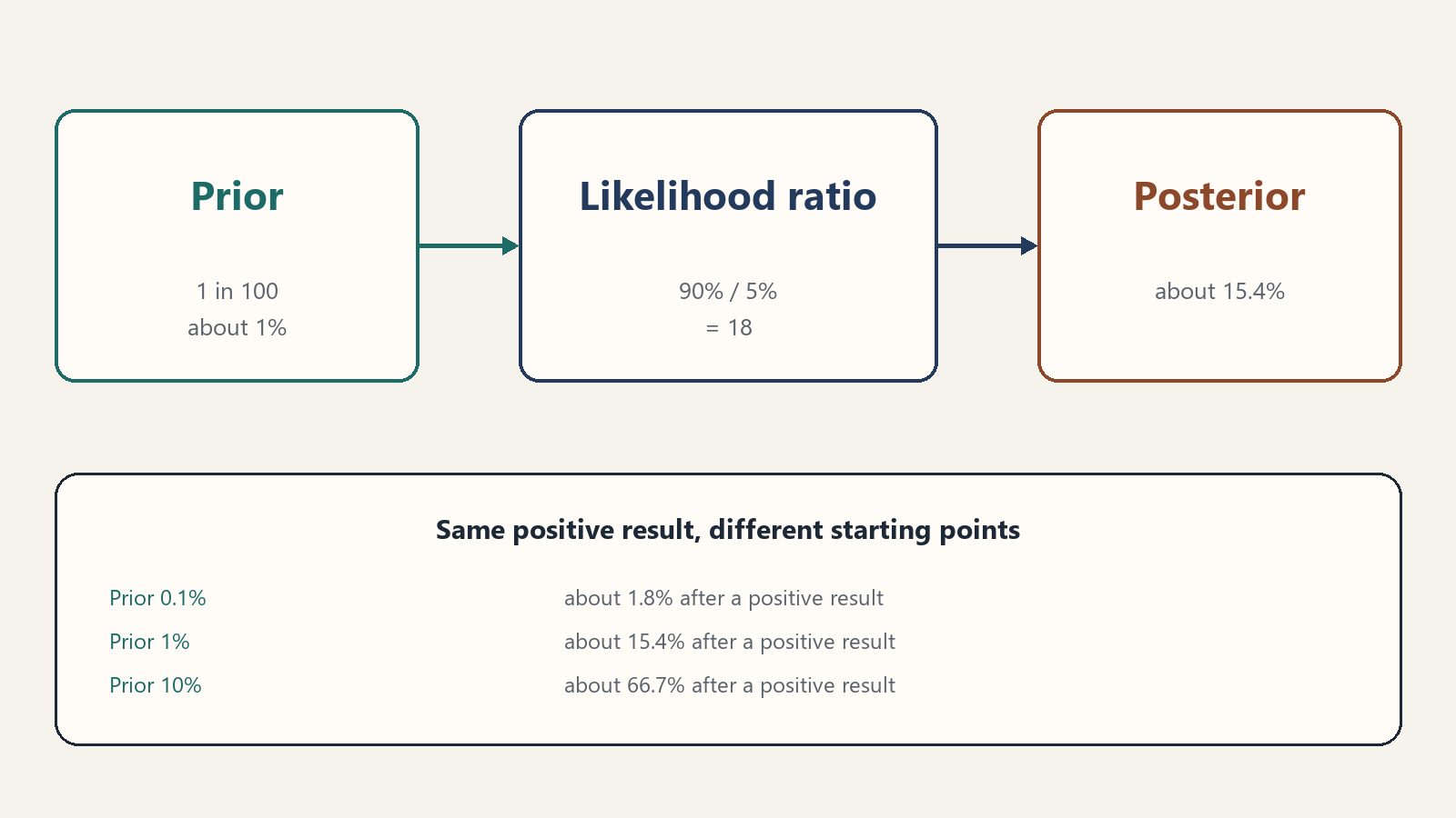
In every row the positive result has the same likelihood ratio, but it leads to a different final assessment. The comparison assumes unchanged sensitivity and specificity. In a real application one has to check whether that assumption is justified for the groups being compared.

That is why the information "the test detects ninety percent of cases" is not enough to interpret a positive result. We also need the false-positive rate among people without the disease, and a justified probability before the test.

How to justify the starting assessment

Here the convenience of a classroom example ends. In practice it is not always clear which comparison group the case belongs to.

Should the starting assessment rest on the frequency of the disease in the whole population, in a defined age group, or among people with similar symptoms? Each of those groups can be the right one for a different range of available information. Using a broad average despite knowledge of particular risk factors can go wrong. So can picking a narrow group only because it yields a desired result.

In a Bayesian analysis the starting point should have a justification. It helps to say which data it comes from, why they apply to our case, and what happens if we adopt other reasonable values. If a small change in the assumptions reverses the conclusion, the reader should know that.

Such sensitivity checks and model assessment belong to a wider process of analysis. Andrew Gelman and coauthors describe in Bayesian Workflow not only the calculation of distributions after the data are in, but also building models, checking them, comparing them, and revising them. The piece is a methodological preprint from 2020, available as arXiv:2011.01808.

A starting assessment can rest on earlier studies, a model, or justified expert knowledge. Putting it into the formula does not remove uncertainty or subjective choices. The arithmetic makes those assumptions visible. Two people can then see whether they differ about the earlier evidence, about the credibility of the new information, or about the model of the phenomenon itself.

How much information a second test adds

After a positive result we run a second test. To show a simple calculation first, assume it has the same sensitivity and specificity as the first, and that the results are conditionally independent both among people with the disease and among people without it. That means that in each of those two groups, knowing the first result does not change the probability of the second. In our model, after the first positive the second test is still positive for 90 percent of people with the disease and for 5 percent of people without it. We are not assuming that we know the person's health: we are describing how the tests behave separately in each group. That independence does not follow automatically from collecting another sample or from using another method. Pishro-Nik treats conditional independence in section 1.4.4 of the same textbook.

If the second test is also positive, under those assumptions we multiply the odds by eighteen again: one over 99, times 18, times 18, equals 324 over 99. The probability of disease is then 324 divided by 324 plus 99, or about 76.6 percent.

This time the presence of the disease is more probable than its absence. The figure of 76.6 percent belongs to our model exactly, not to any pair of positive tests whatever.

What if the "second confirmation" is simply the same result shown in an app and on a laboratory printout? When we know that both messages report one study, the copy is not another measurement. Multiplying the odds by eighteen again would count the same evidence twice.

Between an independent test and an identical copy there are many intermediate cases. Imagine that both tests also react to the same substance unrelated to the disease under study. A person for whom that substance produced the first false positive may receive a second for the same reason. The second result can still carry information, but its weight has to be judged in light of the first. A different method can reduce shared causes of error, but difference of method alone does not prove independence.

The general rule stays simple: we ask what the second result adds beyond what we already know from the first. Mathematically we compare the probability of the second result given the disease with its probability given the absence of the disease, in each case taking the first result into account. Under conditional independence and equal sensitivity and specificity we can reuse the original likelihood ratio. Otherwise we need the ratio that belongs to the second test after the first.

The same question is worth asking when reading the news. Ten outlets can quote one bulletin. Their agreement then tells us mainly how widely the message has spread. Whether the desks independently checked its content requires tracing the sources.

If the second result contradicts the first

Return to our simplified model: two tests with the same parameters and conditionally independent results. The first result is positive, but the second is negative. What then?

A negative result occurs in ten percent of people with the disease and ninety-five percent of people without it. Its likelihood ratio is therefore 0.10 divided by 0.95, or about 0.105. It is less than one, so multiplying the current odds by it lowers the assessed probability of disease.

The odds after the first result were 18 to 99. Multiplying by 0.10 over 0.95 and converting again to a probability yields about 1.9 percent. The assessment therefore falls from 15.4 percent, but it does not return exactly to the original 1 percent. A positive and a negative need not cancel like a vote for and a vote against: each has a different weight set by the study's parameters.

Absence of an expected trace should be read the same way. Failure to detect a trace counts against a hypothesis when that failure is less probable if the hypothesis is true than if the alternative under consideration is true. The meaning of a negative result therefore depends both on the measurement's ability to detect the phenomenon and on what we expect when the phenomenon is absent. If non-detection is nearly as likely in both situations, it does little to tell them apart.

In our example we also assume that the presence or absence of the disease did not change between the tests, and that the test parameters still apply. If the person's condition changed over time, or if treatment affected what the tests measure, we need a model that includes those changes.

Changing an assessment need not mean rejecting a hypothesis

One reading of the screening arithmetic is that a large update of probability need not flip a diagnosis. In debate it is easy to reduce belief to two positions: I accept, or I reject. Often the most important response to new evidence is a shift in the assessment without crossing to the other side.

Raising the estimated probability of disease from one to fifteen percent is a substantial response to the information. The absence of the disease remains more probable. There is no contradiction in that, and no ignoring of the result. The 50 percent line only says which of two possibilities is more probable; it does not by itself set a threshold for diagnosing a disease or for taking action.

A person already attached to a hypothesis can likewise weaken that attachment under a counterargument without discarding the hypothesis at once. A useful discussion should allow that kind of reply. Otherwise every correction becomes a public change of camp, which makes a calm reading of the data harder.

It helps to say in advance what observation would raise our confidence in a hypothesis and what would lower it. If every possible result can only reinforce the view we already hold, it is hard to say that the view is really being tested.

We need not assign every opinion an exact percentage. "This result clearly raises my confidence, but it does not decide between two explanations" can be more honest than an unsupported "I am 83 percent sure."

The model may need revision too

So far we have assumed that we know the frequency of the disease and the parameters of the test. Suppose we begin studying another population, or the way samples are prepared changes. The assumptions we have used may stop describing the new situation.

If every observation is read only as evidence for or against the disease, we can miss the question of whether the method of measurement itself is reliable. More data then do not automatically yield a better description.

Gelman and Cosma Rohilla Shalizi stress in Philosophy and the practice of Bayesian statistics (doi: 10.1111/j.2044-8317.2011.02037.x) that statistical practice needs critical checking of the model. Comparing its predictions with observations is meant to show how the model fails and what should be improved. Computing the posterior, the description of probabilities after the data are included, does not finish that work. The paper appeared in the British Journal of Mathematical and Statistical Psychology in 2013, after online publication in 2012.

In our example one can compare the predicted frequency of positive results with the observed one, and compare test results with an independent assessment of disease presence in a suitably chosen group. Checking only people with a positive result will not show how many cases the test missed. Departures from the predictions will not immediately name the cause, but they will justify another look. Both the assessment of a single case and our knowledge of the test and the population under study may need updating.

That limit matters for broad public disputes as well. The list of explanations under consideration can be incomplete, the data selectively chosen, and the links among sources unrecognized. An elegant calculation will not repair those problems without further work on the assumptions.

Knowing and deciding are two different jobs

After a positive result, should another test be done? The figure 15.4 percent alone does not answer that.

In our hypothetical case further diagnosis could be justified if it would detect a serious disease and if the test itself imposed little burden. An invasive procedure with material risk would be judged differently. One has to weigh the harm of missing the disease, the benefit of finding it, the risk of further tests, and the consequences of a wrong diagnosis. There is no single probability threshold that fits every such decision.

Ordering a confirmatory test is not the same as diagnosing the disease. One can have a sound reason for further checking and still lack the grounds to treat the diagnosis as established. A decision to treat likewise requires the expected benefits and harms of treatment, not only the word "positive" on the report.

The distinction also protects public argument. A decision taken under uncertainty does not prove that the uncertainty has disappeared. And the lack of full certainty does not mean that every decision must be postponed indefinitely.

The question worth taking away

Bayesian reasoning can begin without a calculator. Faced with new information, it helps to say exactly what the hypothesis is, what the earlier assessment rested on, and whether the observed signal would have been equally easy to obtain under a competing explanation. Then check whether the information is really new, and whether it comes from a process we can evaluate.

The central question is: how probable is this result under my hypothesis, and how probable is it under a competing explanation? If the ratio of those probabilities is close to one, the result changes the odds of one hypothesis relative to the other very little, however striking it sounds.

The printout still says "positive." We no longer read it as a finished diagnosis. We can see how the result changed the assessment, which assumptions support that change, and why a further test may add a great deal, a little, or nothing new. The mathematics does not replace judgment. It helps show which conclusions follow from the data and which still need a justification.

The screening example, the disease frequency, and the parameters of both tests are hypothetical. They do not describe a real disease, product, or recommended diagnostic path. The percentages are rounded to one decimal place under the stated assumptions. For the two-test calculation we kept the presence or absence of disease unchanged, gave both tests the same sensitivity and specificity, and treated their results as conditionally independent in both groups. The counts are expected values, not clinical data. Mentions of news and public debate illustrate the logic only.